Eigenvalue level repulsion
Imaging we have two matrices ${\bf A}, {\bf B}$ $\in \mathbb{R}^n$, that are both symmetric. Then, we know that both matrices have $n$ eigenvalues (multiplicity). Let’s start now, gradually morphing ${\bf A}$ to ${\bf B}$ using the following formula
$$ {\bf A}[t] = (1 - t) {\bf A} + t {\bf B}, $$
where $t \in [0, 1]$. What will happen is that matrix ${\bf A}$ will have multiple eigenvalues with probability zero, given we have chosen the matrices properly from the set of all real symmetric matrices. In other words, there will be no time $t$ when matrix ${\bf A}$ won’t have $n$ eigenvalues. We can see an example in Figure $1$ below.
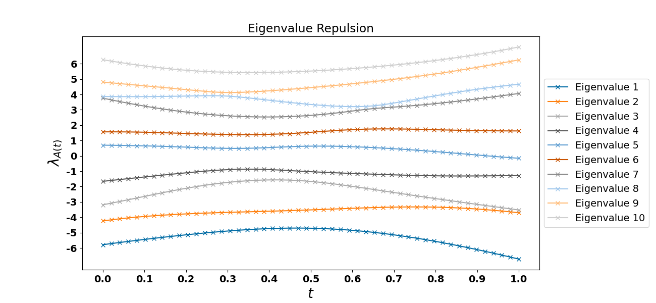
Figure 1. Eigenvalue level repulsion. Notice that as we move from $t=0$ to $t=1$ the eigenvalues of matrix ${\bf A}$ morph to those of ${\bf B}$ and at any instance matrix ${\bf A}$ has $10$ eigenvalues (see the dimension of the matrix ${\bf A}$ in the code snippet below, which is $10$).
The Python code below shows how one can compute the eigenvalue level repulsion.
 1import numpy as np
 2import matplotlib.pylab as plt
 3import matplotlib.style as style
 4
 5style.use('tableau-colorblind10')
 6
 7params = {'font.size': 14,
 8          }
 9plt.rcParams.update(params)
10
11
12def keig(A, k):
13    # Compute the eigenvalues of a matrix, sort them and then choose the k fisrt of them
14    kth_eig = np.sort(np.linalg.eigvals(A))[k]
15    return kth_eig
16
17
18if __name__ == '__main__':
19    np.random.seed(1)
20
21    # Randomly select two matrices A and B and make sure they are symmetric
22    n, nnodes = 10, 50
23    A = np.random.randn(n, n)
24    A = A + A.conj().T
25    B = np.random.randn(n, n)
26    B = B + B.conj().T
27
28    # Define the discretization of interval [0, 1]
29    t = np.linspace(0, 1, nnodes)
30
31    # Run over t and compute the eigenvalues
32    res = []
33    for k in range(n):
34        tmp_mat = []
35        for i in range(nnodes):
36            tmp_mat.append(keig((1 - t[i]) * A + t[i] * B, k))
37        res.append(tmp_mat)
38
39    # Plot the results
40    min_ = int(min(min(res)))
41    max_ = int(max(max(res)))
42
43    fig = plt.figure(figsize=(13, 6))
44    ax = fig.add_subplot(111)
45    for i in range(n):
46        # label numbering should start from 1 not 0
47        ax.plot(t, res[i], '-x', label="Eigenvalue "+str(i+1))
48    ax.set_xlabel(r"$t$", fontsize=20, weight="bold")
49    ax.set_ylabel(r"$\lambda_{A(t)}$", fontsize=20, weight="bold")
50    ax.set_xticks([i/10 for i in range(11)])
51    ticks = ax.get_xticks()
52    ax.set_xticklabels(ticks, fontsize=14, weight='bold')
53    ax.set_yticks([i for i in range(min_, max_)])
54    ticks = ax.get_yticks()
55    ax.set_yticklabels(ticks, fontsize=14, weight='bold')
56
57    pos = ax.get_position()
58    ax.set_position([pos.x0, pos.y0, pos.width * 0.9, pos.height])
59    ax.legend(loc='center right', bbox_to_anchor=(1.25, 0.5))
60
61    ax.set_title("Eigenvalue Repulsion")
62    plt.show()