How do we compute a Gramian Angular Field (GAF) for time series?
Here, we briefly introduce the Gramian Angular Field (GAF) method proposed by [1] to convert time series into images without losing much information. Thus, we can use those images with deep neural networks and computer vision methods to analyze or classify time series. Following [1], we present the main idea behind GAF: to obtain a matrix of similarities between temporal data points of a time series. To do so, the authors in [1] introduced the following algorithm:
![Figure 1. Gramian Angular Field Algorithm (see [1] for more details).](/images/gaf_algo.png)
Figure 1. Gramian Angular Field Algorithm (see [1] for more details).
In Algorithm 1, the variable $t$ represents the time index (time stamp) of the input time series $X$, and the parameter $N$ is a constant factor that determines the span of the polar coordinates. The transformation from the Cartesian to Polar coordinates has two nice properties [1]:
- The transformation is bijective since $\cos(\phi)$ is monotonic when $\phi \in [0, \pi]$, and thus the transformation returns unique representations in the polar coordinates along with a unique inverse transform.
- Polar coordinates preserve absolute temporal relations.
Furthermore, the authors in [1] show that we can obtain the GAF matrix ${\bf G}$ by using a modified inner product (penalized inner product). More precisely, ${\bf G} = \hat{{\bf X}}^{\intercal} \cdot \hat{{\bf X}}- \sqrt{{\bf I} - \hat{\bf X}^2}^{\intercal} \cdot \sqrt{{\bf I} - \hat{{\bf X}}^2} $, where ${\bf I}$ is a unit row vector. Therefore, we can obtain the matrix {\bf G} as a Gram matrix based on the inner product $<x, y> = x \cdot y - \sqrt{1 - x^2} \cdot \sqrt{1 - y^2}$, and hence $G_{ij} = <\hat{x}_i, \hat{x}_j>$, where $\hat{x}_i$ is a normalized temporal data point.
In general, a Gram (or Gramian) matrix is a matrix ${\bf G} \in \mathbb{R}^{m \times m}$ with elements $G_{ij} = <{\bf v}_i, {\bf v}_j> $ (inner product), where $v \in \mathbb{R}^m$. Another way to express matrix ${\bf G}$ is as ${\bf G} = {\bf X}^{\dagger} {\bf X}$, where the vector ${\bf v}_1, \ldots, \bf{v}_m $ are the columns of ${\bf X}$.
Below, we give a snippet of Python code that implements Algorithm 1.
The first step is to store the time series into an array and then normalize the values into $[-1, 1]$ using the MinMaxScaler of sklearn. Then we compute the angle $\theta = \arccos({\bf x})$, where ${\bf x}$ is the vector that contains the time series data points and the $r$ and finally the matrix ${\bf G}$ based on the angles $\phi_i$.
 1import numpy as np
 2from sklearn.preprocessing import MinMaxScaler
 3
 4def estimateGAF(x):
 5    scaler = MinMaxScaler(feature_range=(-1, 1))
 6    x = scaler.fit_transform(x.reshape(-1, 1))
 7
 8    theta = np.arccos(x)
 9    r = np.linspace(0, 1, len(x))
10
11    def cos_(x, y):
12        return np.cos(x + y)
13
14    res = np.vectorize(cos_)(*np.meshgrid(theta, theta, sparse=True))
15    return res, theta, r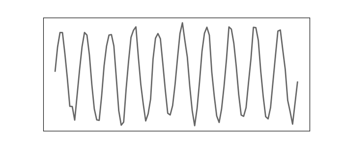
Figure 2. A sinusoidal signal with additive white noise.
As an example, we consider the signal shown in Figure 2 as our time series, and we apply the function estimateGAF to it. The polar representation is shown in Figure 3, and the corresponding GAF matrix in Figure 4.
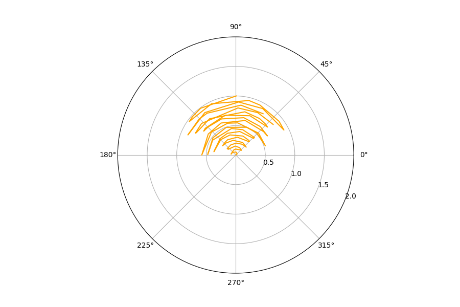
Figure 3. Polar representation of signal shown in Figure 2.
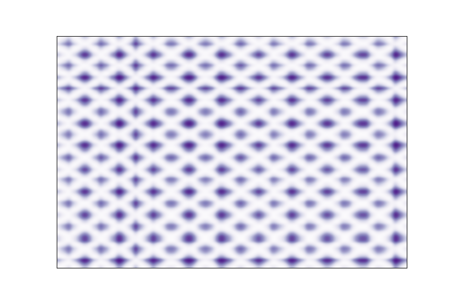
Figure 4. GAF matrix ${\bf G}$ for the signal shown in Figure 2.
GAF expresses some interesting properties:
- It preserves the temporal dependencies.
- Time increases as the position moves from top-left to bottom-right.
- A GAF matrix contains temporal correlations.
- The main diagonal $G_{i,i}$ contains the original angular information.
References
- Z. Wang, and T. Oates, Encoding Time Series as Images for Visual Inspection and Classification Using Tiled Convolutional Neural Networks, In Workshops at the twenty-ninth AAAI conference on artificial intelligence (Vol. 1, pp. 1-7).