An introduction to self-organizing maps
This post presents the classical self-organizing map algorithm proposed by Grossberg [1] and Teuvo Kohonen [2]. We explain the algorithm’s fundamental aspects and applications and offer a basic implementation in Pytorch.
Introduction
Let us begin with a prevalent problem in science. We often have to deal with data that live in a high-dimensional space $\mathcal{X} \in \mathbb{R}^k$. When $k > 3$, things get rough for people who need help to visualize what’s happening. Moreover, many algorithms cannot operate fast enough in high-dimensional spaces [3, 4]. Therefore, we rely on methods that reduce the dimensionality without compromising or losing much information.
One such method is a self-organizing map or SOM. SOM is an unsupervised learning algorithm that maps a high-dimensional space into a lower-dimensional one through an artificial neural network. In a more mathematical context, the idea behind an unsupervised learning problem and mainly a self-organizing map, is to learn the input distribution, meaning we are looking at an approximation for the joint distribution $p(x, y)$, where $x$ represents input samples and $y$ the output, without making any assumptions about causality.
Applications
We have already seen the dimensionality reduction problem, where the data we handle are usually high-dimensional, rendering their analysis, processing, or interpretation hard. Therefore, we can use a SOM to map the original input space to a low-dimensional space and work with the reduced data [2]. Another feature of the SOM is that it retains the topographic properties of the input distribution (space). The code words are topographically organized, meaning that the neighboring units of the map represent data that are nearby in the input space. For instance, classifying world poverty is a problem where clusters (or groups of units/neurons) represent poor, rich, or in-between countries [http://www.cis.hut.fi/research/som-research/worldmap.html]. There are many other applications, but providing an exhaustive list is out of the scope of this post.
Notation and Terminology
Before diving into the details and implementing the SOM algorithms, we must define some mathematical quantities and determine out terminology. The SOM is implemented as a neural network $\mathcal{F}({\bf \theta})$ that maps a high-dimensional manifold $ \mathcal{X} \in \mathbb{R}^k $ to a low-dimensional predefined lattice $\mathcal{Y} \in \mathbb{R}^m$, where $ m \ll k $. The input to the SOM is a vector $ {\bf x} \in \mathcal{X} $, and the weights, $ {\bf w} $, of the neural network that learns the representations are called code words and the set of the code words, $ \mathcal{W} = {\bf w_1, \ldots, w_n} $, is called a codebook. The cardinal number of $\mathcal{W}$ is the number of units we use in the low-level lattice or the number of neural network units. We let $ d(\cdot, \cdot) $ be the Minkowski distance defined as $$ d({\bf x}, {\bf y}) = \Big( \sum_{i=1}^{k} |x_i - y_i|^p \Big)^{\frac{1}{p}}, \qquad (1) $$ where here ${\bf x}, {\bf y} \in \mathbb{R}^n $ and $ p \geq 1$. For different values of $ p $, we recover different known distance functions such as the Euclidean distance ($p=2$) or the Manhattan ($p=1$).
The SOM Algorithm
We are now ready to introduce the SOM algorithm. First, we will describe the main idea behind the SOM algorithm in plain words, and then we will give the pseudocode and its implementation along with some examples.
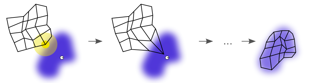
Figure 1. Illustration of SOM algorithm steps. At the beginning (t=0), we see that the winner unit (BMU, center of yellow disc) that is closer to the current sample (white disc) has been identified. The SOM algorithm adjusts the codebook based on a neighborhood function (yellow disc) so the map will come closer to the sample. After all the iterations had been exhausted, the SOM learned the representation (black grid) of the input distribution (blue cloud). This figure is licensed under the Creative Commons Attribution-Share Alike 3.0 Unported (Wikipedia).
The first step is to initialize the codebook; we usually do that by assigning random values to the code words. Once we initialize the codebook, we start the learning iteration. At each iteration or epoch, we draw a sample ${\bf x}$ from the input space $ \mathcal{X} $ and compute the distance of that sample from all the code words. We select the code word with the smallest distance from ${\bf x}$ such that $$ i_{\text{BMU}} = \text{BMU} = \text{arg}\min_{i\in \mathbb{N}^+} \left\{ d({\bf x}, {\bf w}^t_i) \right\}, \qquad (2) $$
and we call that unit (neuron) the best matching unit (BMU) or the winner unit.
Figure 1 shows a random initialization of the codebook (black grid) that contains two-dimensional code words ($ \mathcal{X} \in \mathbb{R}^2$). The white disc represents the sample ${\bf x}$ we drew. After we compute all the distances between that sample and all the grid points, we observe that the closest point of the grid to that sample is the one at the center of the yellow disc.
So now the next step is to update the code words ${\bf w}_i$ ($i = 1, \ldots, n$) by moving them towards the sample ${\bf x}$ according to the following equation:
$$ {\bf w}_i^{t+1} = {\bf w}_i^t + \epsilon(t) h(t, \text{BMU}, \sigma(t))({\bf x} - {\bf w}_i^t), \qquad(3) $$
and updating the code words that fall within a neighborhood defined by the function:
$$ h(t, \text{BMU}; \sigma(t)) = \exp\Big( \Big( \frac{d({\bf w}^t_{\text{BMU}}, {\bf w}^t_i)}{\sigma(t)} \Big)^2 \Big), \qquad(4) $$
where $t$ is the current iteration (or time step or epoch). $\epsilon(t)$ and $\sigma(t)$ are the time-dependent learning rate and neighborhood function’s variance, respectively. They both decay exponentially based on $ z_i \Big( \frac{z_f}{z_i} \Big)^{\frac{t}{t_f}} $, where $z_i$ and $z_f$ are the initial and final values, respectively ($z = {\epsilon, \sigma}$). We assume $z_i \gg z_f$ for the initial and final values. The idea behind a time-dependent decaying learning rate is to freeze learning after some time, and a decaying variance of the neighborhood function guarantees that as the learning progresses, the number of units that get to update their weights decreases. Moreover, at the beginning of learning, the radius of the neighborhood function should be large enough. At the end of learning, we should keep the radius small such that only one or zero neighbors are within the immediate vicinity of the BMU.
Figure 2 shows the pseudocode of the SOM algorithm. The algorithm presented here is an online learning algorithm (or sequential), meaning that one sample of data is processed at each iteration. A different version of the SOM algorithm runs offline and uses the entire data set at each iteration, called batch SOM. In this post, we will implement the online algorithm used in our examples.
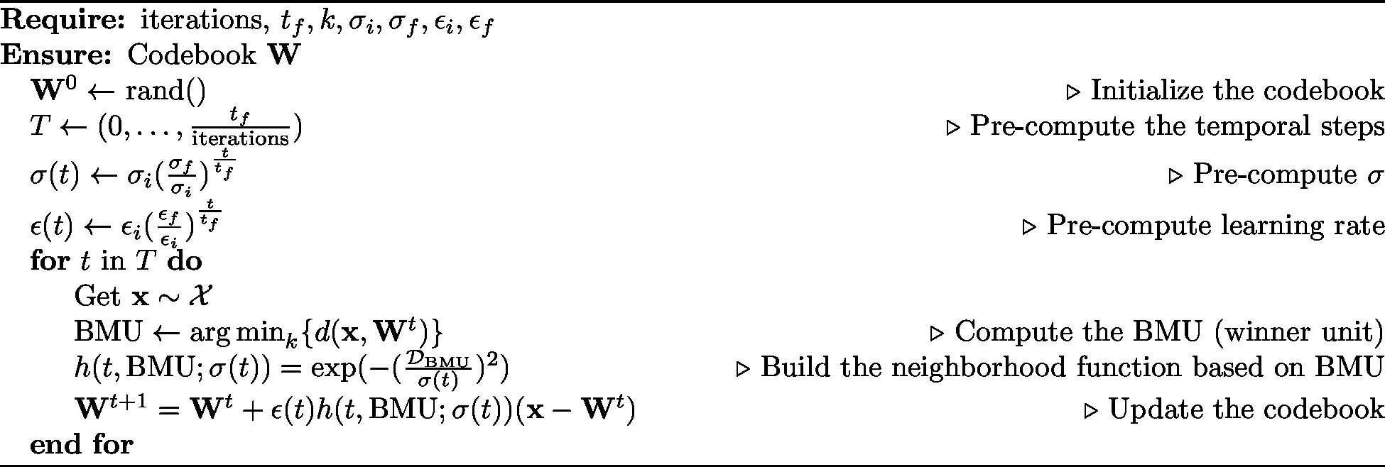
Figure 2. Self-organizing map basic algorithm.
Pytorch Implementation
The source code below implements the SOM algorithm given in Figure 2. It is a simple translation of the pseudocode to Python. In this implementation, we contain all the parameters and the codebooks in $[0, 1]^k$, where $k \in \mathbb{N}^+$. We also consider the neighborhood function a Gaussian, and the final time $t_f = 1$. The metric $d(\cdot, \cdot)$ is the Euclidean distance ($p=2$ in Equation 1).
 1import numpy as np
 2import matplotlib.pylab as plt
 3
 4import torch
 5from torch import nn
 6
 7
 8class SOM(nn.Module):
 9    def __init__(self,
10                 n_units=16,
11                 dim=2,
12                 iters=1000,
13                 lrate=(0.5, 0.01),
14                 sigma=(0.5, 0.01)):
15        super().__init__()
16        self.n_units = n_units				# Number of units (n in main text)
17        self.dim = dim						# Code words dim (k in main text)
18        self.iters = iters
19        self.lrate_i = lrate[0]
20        self.lrate_f = lrate[1]
21        self.sigma_i = sigma[0]
22        self.sigma_f = sigma[1]
23
24		# Initialize the code words
25        self.initCodebook()
26
27		# Initialize a two-dimensional grid
28        self.initLatice()
29
30		# Pre-compute the time array, learning rate, and variance
31        self.t = torch.linspace(0, 1, steps=iters)
32        self.lrate = self.lrate_i * (self.lrate_f / self.lrate_i)**self.t
33        self.sigma = self.sigma_i * (self.sigma_f / self.sigma_i)**self.t
34
35    def initCodebook(self):
36    	""" Initialize the code words using random values drawn from a
37    	uniform distribution in [0, 0.01).
38    	"""
39        self.codebook = torch.ones([self.n_units*self.n_units, self.dim])
40        nn.init.uniform_(self.codebook, a=0, b=0.01)
41
42    def initLatice(self):
43    	""" Initialize a two-dimensional grid (latice) on which units
44    	(or neurons) are placed. Moreover, computes the distances between all
45    	the pairs within the grid.
46
47    	"""
48        line = torch.linspace(0, 1, steps=self.n_units)
49        grid_x, grid_y = torch.meshgrid(line, line, indexing="ij")
50        p = torch.cat((grid_x.flatten().reshape(-1, 1),
51                       grid_y.flatten().reshape(-1, 1)), dim=1)
52        self.dist = torch.cdist(p, p)
53
54    def fit(self, X):
55    	""" Fit the input data X to a two-dimensional SOM.
56    	"""
57        for t in range(self.iters):
58
59        	# Sample the input space
60        	x = X[np.random.randint(X.shape[0])]
61
62			# Find the BMU
63            BMU = torch.argmin((((self.codebook - x))**2).sum(dim=-1))
64
65			# Compute the neighborhood function
66            h = torch.exp(-(self.dist[BMU]/self.sigma[t])**2).unsqueeze(1)
67
68			# Update the codebook
69            self.codebook -= self.lrate[t] * h * (self.codebook - x)
Examples
![Figure 3. Self-organizing maps. (A) Shows a self-organizing map of the unit square $[0, 1]^2$, and (B) shows a a map for a ring in $[-1, 1]^2$.](/images/som_maps.png)
Figure 3. Self-organizing maps. (A) Shows a self-organizing map of the unit square $[0, 1]^2$, and (B) shows a a map for a ring in $[-1, 1]^2$.
Square in $ \mathbb{R}^2 $
Our first example is to map a two-dimensional rectangular distribution in the $[0, 1] \times [0, 1]$. To this end, we randomly generate points $(x_1, x_2) \in [0, 1] \times [0, 1]$ from a uniform distribution $\mathcal{U}$. After running the code presented earlier for $3000$ iterations and with $\epsilon_i = \sigma_i = 0.5$ and $\epsilon_f = \sigma_f = 0.01$, we obtain the self-organized map illustrated in Figure 3A, where the red dots represent the input space (and thus the samples we used to train our neural network). The white discs are the units of our SOM.
Ring in $ \mathbb{R}^2 $
The second example is again related to space $[0, 1] \times [0, 1] $, only this time we draw uniformly points from a ring, rendering this problem a little bit harder for the SOM algorithm since there is a hole in the center of our distribution. Figure 3B shows the input space distribution in red dots, and again, we see that the SOM algorithm has captured the input space. The code words (white discs) cover the space, and the lattice (black solid lines) are well organized. However, we see some units representing the hole (void) in the middle of the ring. That is a known problem with Kohonen’s SOM algorithm. The parameters for this experiment are the same as before.
Evaluate a SOM
When measuring the quality of a self-organized map, there is no one measure to rule them all. People use many different measures in the literature to measure how good or bad a self-organized map is. Three well-known measures are:
-
The quantization error (or distortion), which is the average distance of the minimum of all the pairwise distances between the input space samples $\mathcal{X}$ and the codebook $\mathcal{W}$, $ \mathcal{E_{Q}} = \mathbb{E}[\min\left\{ \mathcal{D}(\mathcal{X}, \mathcal{W}) \right\} $. The quantization error does not measure how well the map preserves the data’s topology but instead measures the goodness-of-fit of the input distribution by the map. The lower the $\mathcal{E_Q}$, the better.
-
The topographic error quantifies how well the map captures the shape of the input data and how well the topology of the map preserves the input space. The topographic error is computed as $\mathcal{E_{T}} = \frac{1}{|\mathcal{X}|} \sum_{{\bf x} \in \mathcal{X}}^{}I({\bf x}) $, where $I({\bf x}) = 1$ when the BMU and the second best matching unit are not neighbors, and zero otherwise. The lower the value of the $\mathcal{E_{T}}$, the better.
In our examples above, we measure the quantization and topographic errors. As Table 1 shows, the errors for the square distribution are indeed minor, meaning that the maps capture and preserve the topology of the input distribution. However, the quantization error is not that small for the ring distribution, meaning that the map preserves the topology since the topographic error is small. Still, the map needs to fit the data distribution better. We can see that the map also tries to find non-existent data in the ring’s hole.
| Example | $\mathcal{E_Q} $ | $\mathcal{E_{T}}$ |
|---|---|---|
| Square | $0.034$ | $0.028$ |
| Ring | $0.255$ | $0.04$ |
Summary
In this post, we introduced some fundamental ideas of self-organizing maps. We tried to convey how the SOM algorithm works and provided a simple Python implementation using Pytorch. Finally, we tested our implementation on two basic examples: a two-dimensional distribution of a rectangle and one of a two-dimensional disc. In both cases, we see how the SOM algorithm learns the representations and correctly maps the input distribution.
Source Code
The entire source code for the experiments used in this post is freely available here.
Cite as
@article{detorakis2023som,
  title   = "An introduction to self-organizing maps",
  author  = "Georgios Is. Detorakis",
  journal = "gdetor.github.io",
  year    = "2023",
  url     = "https://gdetor.github.io/posts/som"
}
References
- Grossberg S., Physiological interpretation of the self-organizing map algorithm, 1994.
- Kohonen T., Self-organized formation of topologically correct feature maps, Biol Cybern., 1982;43(1):59–69.
- Bellman R. E., Dynamic programming, Princeton University Press, Rand Corporation (1957).
- Bellman R. E., Adaptive control processes: a guided tour, Princeton University Press. ISBN 9780691079011, 1961.
- Ponmalai, R., and Kamath, C., Self-organizing maps and their applications to data analysis, Lawrence Livermore National Lab.(LLNL), Livermore, CA, 2019.