Autocorrelation Functions for Time Series
This post aims to provide some theoretical background on autocorrelation functions and how to use them to analyze time series. Furthermore, we show how to use the Autocorrelation (ACF) function and the Partial Autocorrelation (PACF) function to determine the parameters for an ARMA model.
Brief introduction to time series
In a previous post (see here), we introduced some basic definitions and terminology about time series. We repeat the same definitions here to avoid forcing the reader to move back and forth.
In layperson’s terms, a time series is a series of observations (or data points) indexed in time order [1, 2]. A few examples of time series are
- The daily closing price of a stock in the stock market
- The number of air passengers per month
- The biosignals recorded from electroencephalogram or electrocardiogram
Figure 1 shows the number of air passengers per month from January 1949 to September 1960. We are going to use this dataset in all the examples in this post, so if you would like to try the examples by yourself; you can download the data from Kaggle here.
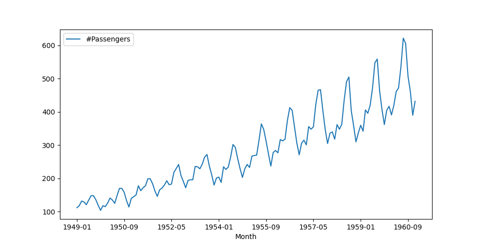
Figure 1. An example of a time series showing the number of air passengers per month.
A more rigorous definition of a time series found in [1] (Chapter 1, pg 1) is given below:
Let $ k \in \mathbf{N}, T \subseteq \mathbf{R} $. A function $$ x: T \rightarrow \mathbf{R}^k, \hspace{2mm} t \rightarrow x_t $$ or equivalently, a set of indexed elements of $ \mathbf{R}^k $, $$ \begin{Bmatrix} x_t | x_t \in \mathbf{R}^k, \hspace{2mm} t \in T \end{Bmatrix} $$ is called an observed time series (or time series). Sometimes, we write $ x_t(t \in T) $ or $ (x_t)_{t\in T} $.
When $ k = 1 $ the time series is called univariate, otherwise is called multivariate. $ T $ determines if the time series is [1]:
- discrete $ T $ is countable, and $ \forall a < b \in \mathbb{R}: T \cap[a, b] $ is finite,
- continuous $ T = [a, b], a < b \in \mathbb{R}, T = \mathbb{R}_{+} \hspace{2mm} \text{or} \hspace{2mm} T = \mathbb{R} $,
- equidistant $ T $ is discrete, and $ \exists u \hspace{2mm} s.t. \hspace{2mm} t_{j+1} - t_j = u $.
From now on and for simplicity’s sake we will use the following notation for a time series: $ \begin{Bmatrix} y[1], y[2], \ldots , y[N] \end{Bmatrix} $, where $ N \in \mathbb{N} $ or $ y[t] $, where $t=1, \ldots , N $.
What is autocorrelation (ACF)
The Autocorrelation function (from now on, we will refer to the autocorrelation function as ACF) for a given time series $ x[t] $ at times $ t_1, t_2, \ldots, t_N $ with mean $ \mu_t $ and the time series $ x[s] $ at time $ s_1, s_2, \ldots, s_N $ with mean $ \mu_s $ is givenb by following formula:
$$ \rho(s, t) = \frac{\mathbb{E}[(x[s]-\mu_s)(x[t]-\mu_t)]}{\mathbb{E}[(x[s]-\mu_s)^2] \mathbb{E}[(x[t]-\mu_t)^2]}. \qquad (1) $$
Another way to express the ACF is through the autocovariance function. By plugging the equation of covariance
$$ \gamma(s, t) = \text{cov}(x[s], x[t]) = \mathbb{E}[(x[s]-\mu_s)(x[t]-\mu_t)], $$ into equation (1) we obtain $$ \rho(s, t) = \frac{\gamma(s, t)}{\sqrt{\gamma(s, s) \gamma(t, t)}}. $$
The above definitions are valid for time series of real numbers. If the time series are complex then we have to replace the term $ \mathbb{E}[(x[s]-\mu_s)(x[t]-\mu_t)] $ with the complex conjugate $\mathbb{E}[(x[s]-\mu_s)\bar{(x[t]-\mu_t)}] $.
From the definitions above one can conclude, first, the autocovariance of a time series with itself is the variance of the signal (i.e., $ \gamma(t, t) = \text{Var}[x[t]] $) and second, the autocorrelation of a time series x[t] with itself is one (i.e., $ \rho(t, t) = 1 $).
Let’s now explain the autocorrelation in layperson’s terms and give some intuition on the information we obtain. Let’s start with the very notion of a time series. In a time series, the data points are ordered temporally. Thus, extra information is stored in a time series, meaning we can determine how past data (historical data) can affect present or future values or the correlation between those points. Therefore, autocorrelation or serial correlation is nothing more than the correlation of a data point with its past values (previous times).
How to compute ACF
Therefore, to estimate the ACF, we start by evaluating the original time series' correlation with itself (zero lag). Then, we introduce a lag into our original time series and estimate the correlation between the original time series and its lagged version. We repeat those steps until we exhaust the predetermined number of lags. The table below shows an example of a time series and its first three lagged signals. From now on, we will use the letter $ k $ to indicate any lag.
| ($ k = 0 $) | $ k = 1 $ | $ k = 2 $ | $ k = 3 $ |
|---|---|---|---|
| 1 | NaN | NaN | NaN |
| 2 | 1 | NaN | NaN |
| 3 | 2 | 1 | NaN |
| 4 | 3 | 2 | 1 |
| 5 | 4 | 3 | 2 |
| 6 | 5 | 4 | 3 |
| 7 | 6 | 5 | 4 |
Let’s now estimate the ACF for the data given in the table above. First, we will write our custom ACF function in the Python programming language, and then we will introduce the ACF function of the statsmodels Python package.
 1>> import numpy as np
 2
 3def rho(x, nlags=1):
 4    # Create a list with all the lagged versions of input signal x
 5    x_lagged = [x[:(len(x) - i)] for i in range(nlags)]
 6
 7    # Compute the mean of input x
 8    x_bar = x.mean()
 9
10    # Initialize a list that contains the correlations for each lag
11    acf = []
12
13    # Loop over all lags and use equation (1)
14    for lag in range(nlags):
15        nominator = ((x[lag:] - x_bar) * (x_lagged[lag] - x_bar)).sum()
16        denominator = ((x - x_bar)**2).sum()
17        acf.append(nominator / denominator)
18    return acf
19
20
21>> x = np.array([1, 2, 3, 4, 5, 6, 7])
22>> rho(x, nlags=4)
23[1.0, 0.5714285714285714, 0.17857142857142858, -0.14285714285714285]1>> from statsmodels.tsa.stattools import acf # import ACF
2
3
4>> x = np.array([1, 2, 3, 4, 5, 6, 7])
5>> acf(x, nlags=3, fft=True)
6array([ 1. , 0.57142857, 0.17857143, -0.14285714])As we expected, the ACF of the statsmodels package returns the same results as our custom-made function does. The only difference is that we used four lags in our custom function, and that’s because we count the zero lag ($ k = 0 $) as well. For more information about the ACF function you can check the docs of statsmodels package.
One important note regarding ACF and later the PACF is the number of lags we have to use. The statsmodels module computes the number of lags using the following formula
$$ \text{nlags} = \min \begin{Bmatrix} 10 \log_{10}(N), N - 1 \end{Bmatrix}, $$
where $ N $ is the number of observations in the time series (raw data).
The ACF is often used to identify non-randomness in a time series and to aid in determining the parameters of a mathematical model for that time series.
What is partial autocorrelation (PACF)
Partial autocorrelation, or PACF, is more challenging to understand than ACF. Let’s understand the intuition behind the PACF, and then we will see how to estimate the PACF for a time series. Remember that the ACF reveals how a measurement (or a data point) at a given time index $ t $ affects a data point at time $ t - k $ ($ k $ is the lag). In that case, the formula for estimating ACF considers all the intermediate data points $ t + 1, t + 2, \ldots, t + k - 1 $ until it reaches the $ t + k $. Now, the PACF ignores the information in the intermediate data points; hence, it is called partial.
Let’s now give a more rigorous mathematical definition of PACF. Assume that we have a time series x[t], then the PACF is defined as
$$ \rho_{\text{partial}}(t, t) = \text{corr}(x[t+1], x[t]) \quad for k = 1, $$
$$ \rho_{\text{partial}}(t, k) = \text{corr}(x[t+k] - \hat{x}[t+k], x[t] - \hat{x}[t]), \quad for k \geq 2, $$
where $ \hat{x}[t+k] $ and $ \hat{x}[t] $ are linear combinations of all the intermediate data points (i.e., $ x[t+1], x[t+2], \ldots, x[t+k-1]$) that minimize the mean squared error (see here) of $ x[t+k] $ and $ x[t] $, respectively.
How to compute PACF
Estimation of the PACF can be done with several algorithms. The most known are (i) the Yule-Walker approach, (ii) the ordinary least squares (OLS), and the Levinson-Durbin recursion method. The package statsmodels implements all those methods and a few more (see statsmodels docs).
Let’s take the previous very simple example and estimate the PCAF for the time series $ x[t] = 1, 2, 3, 4, 5, 6, 7 $.
1>> from statsmodels.tsa.stattools import acf       # import ACF
2
3>> x = np.array([1, 2, 3, 4, 5, 6, 7])
4>> acf(x, nlags=3, method="ols")
5array([ 1.00000000e+00,  1.00000000e+00,  1.55431223e-15, -3.33333333e-01])
In the code snippet above, we specified the algorithm for estimating the PCAF
to be the ordinary least squares. It is relatively simple to implement the OLS
method from scratch. We will use the function lagmat of statsmodels, which
creates a $ 2d $ array of lags, and we will separate the zero lag signal,
which is the original data. Finally, we will use the Numpy function lstsq
to estimate the parameters of the least squares and thus compute the PACF.
 1>> import numpy as np
 2>> from numpy.linalg import lstsq
 3>> from statsmodels.tsa.stattools import lagmat
 4
 5>> x = np.array([1, 2, 3, 4, 5, 6, 7])
 6
 7# Compute the lags (x_lagged) and keep the original time series in x0
 8>> x_lagged, x0 = lagmat(x, 3, original="sep")
 9
10# Prepend x_lagged with a column of ones (add constant)
11>> x_lagged = x_lagged = np.append(np.ones((7,1)), x_lagged, axis=1)
12
13# The first element of PACF is always 1.0
14pacf = [1.0]
15
16# Run the least squares over lags
17>> for lag in range(1, lags + 1):
18>>     params = lstsq(x_lagged[lag:, :(lag+1)], x0[lag:], rcond=None)[0]
19>>     pacf.append(params[-1][0])
20
21>> print(pacf)
22[1.0, 1.000000000000001, 1.5543122344752192e-15, -0.33333333333333415]
Remember that we used the least squares method. If we had used a
a different approach to estimate the PACF, the values would
differ from the ones in the code snippet above. Moreover, the function
lstsq receives an argument named rcond, a cut-off ratio
for small singular values of x_lagged.
Visualization of ACF and PACF
We have now defined ACF and PACF and learned how to estimate them
given a time series. Now, we will explore the visualization of ACF and PACF
and learn how to interpret their graphical representations. To better
demonstrate the power of ACF and PACF visualization, we will apply those
two methods to the airport passengers’ data set (see Figure 1).
We will use the functions plot_acf and plot_pacf provided by the
Python module statsmodels to simplify things.
 1import numpy as np
 2import matplotlib.pylab as plt
 3
 4# Import the plot_acf, and plot_pacf functtions
 5from statsmodels.graphics.tsaplots import plot_acf, plot_pacf
 6
 7# Load the data
 8x = np.genfromtxt("PATH_TO_FILE/passengers.csv")
 9
10fig = plt.figure(figsize=(9, 12))
11ax1 = fig.add_subplot(211)
12
13# Call the function for estimating and plotting the ACF
14plot_acf(x, ax1, fft=True)
15
16ticks = ax1.get_xticks().astype('i')
17ax1.set_xticklabels(ticks, fontsize=14, weight='bold')
18ticks = ax1.get_yticks()
19ax1.set_yticklabels(ticks, fontsize=14, weight='bold')
20ax1.set_title("Autocorrelation (ACF)", fontsize=16, weight='bold')
21
22ax2 = fig.add_subplot(212)
23
24# Call the function plot_pacf to estimate and visualize the PACF
25# We use the method "ols" as we did in a previous example
26plot_pacf(x, ax2, method="ols")
27
28ticks = ax2.get_xticks().astype('i')
29ax2.set_xticklabels(ticks, fontsize=14, weight='bold')
30ticks = ax2.get_yticks()
31ax2.set_yticklabels(ticks, fontsize=14, weight='bold')
32ax2.set_title("Partial Autocorrelation (PACF)", fontsize=16, weight='bold')
33plt.show()
After running the script above, we get the plots of ACF and PACF, as depicted in Figure 2. The left panel shows the ACF, and the right is the PACF. Blue-shaded areas indicate the confidence interval cone; each point outside is considered significant ($ 95 $% confidence). But, whatever is within that cone is regarded as zero.
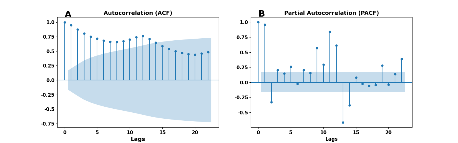
Figure 2. ACF and PACF on airport passengers data set. Left panel - ACF, right panel PACF.
We observe that the first component in the ACF and PACF plots is equal to one, as we expected (and have already discussed). A second apparent observation is the reflection of the original’s data periodicity in the ACF plot. The most important part of those graphic representations is the number of statistically significant correlations (outside the cone). Data points in the ACF plot reflect the correlation between a data point in our time series and its past values. Therefore, the number of significant correlations indicates how far in the past one should look to predict a future point using some mathematical/statistical model.
In the following sections, we will learn how to use the ACF and PACF plots to make assumptions about our models and determine their parameters.
What is an ARMA and an ARIMA model?
We will begin our discussion on ARMA and ARIMA models by introducing the autoregressive (AR) and the moving average (MA) models.
Autoregressive Model - AR(p)
The AR(p) model is based on linear regression. It assumes that the current value $ x[t] $ is dependent on previous (past) values (observations). Due to this ``linear’’ relationship to the past, AR(p) relies on linear regression. More precisely, it is described by the following equation:
$$ x[t] = \sum_{i=1}^{p} \phi [i] x[t-i] + \epsilon [t], \qquad (2) $$
where $ \phi[1], \ldots, \phi[p] $ are the parameters of the model, and $ \epsilon[t] $ is white noise. We will refer to equation (2) as AR($ p $) or AR of order $p$. The order $ p $ controls how many terms in the right-hand side of equation (2) will contribute to the estimation of $ x[t] $.
Moving Average Model - MA(q)
On the other hand, the MA(q) model relies on past error terms to estimate the current value $ x[t] $, and it is given by
$$ x[t] = \mu + \sum_{i=1}^{q} \theta[i] \epsilon[t - i] + \epsilon[t], \qquad (3) $$
where $ \mu $ is the mean of the time series (all observations up to $ t - 1 $), $ \theta[1], \ldots, \theta[q] $ are the parameters of the model, and $ \epsilon[t], \epsilon[t-1], \ldots, \epsilon[t-q] $ are white noise error terms. Because the error terms are white noise, no linearity is involved in the MA(q) model as in the AR(p) model. The parameter $ q $ is the order of the MA(q) model and determines how many terms the value $ x[t] $ will depend on.
Autoregressive-moving-average - ARMA(p, q)
In the case where we combine an AR(p) model with a MA(q), we obtain an autoregressive-moving average model, ARMA(p, q). In the ARMA(p, q) model, $ p $ is the autoregressive order, and $ q $ is the order of the moving average. ARMA(p, q) model is described by:
$$ x[t] = \epsilon[t] + \sum_{i=1}^{p} \phi[i] x[t-i] + \sum_{i=1}^{q} \theta[i] \epsilon[t-i]. \qquad (4) $$
Lag (L) and backshift (B) operators. In a time series context, the backshift operator acts on a time series element and returns the previous element as its name reveals. For instance, if $ x[t] = \begin{Bmatrix} x[1], x[2], \ldots, \end{Bmatrix} $ is a time series then $ Bx[t] = x[t-1] $ for each $ t > 1 $. The lag operator $ L $ acts in the same way $ Lx[t] = x[t-1] $. Furthermore, we can raise both operators in integer powers, $ L^k x[t] = x[t-k] $.
Another way to write equation (4) is to use the lag operator, and thus $$ \Big(1 - \sum_{i=1}^{p} \phi[i] L^i \Big) x[t] =\Big(1 + \sum_{i=1}^{q} \theta[i] L^i \Big) \epsilon[t]. $$
Stationarity A wide-sense stationary time series has a constant mean and variance (autocovariance) over time. For instance, the passengers' data in Figure 1 are non-stationary since an upward trend indicates that the mean increases over time. However, because the variance does not change, we will call that time series non-stationary in the sense of mean. You can find more details about stationarity here and in [1].
Differencing The time series in Figure 1 are non-stationary in the sense of mean (see Stationarity). One way to eliminate the non-stationarity is to apply a differencing transform, $ x^{\prime}[t] = x[t] - x[t-1] $ (for instance, in Python, we could use the
diff()function to apply the differencing transform on the original time series.
Autoregressive Integrated Moving Average - ARIMA(p, d, q)
ARIMA(p, q, d) is a generalzation of ARMA(p, q) model. ARIMA can be seen as an improvement of ARMA for time series that show non-stationarity in the sense of mean. The integrated part of the ARIMA model corresponds to the differencing of the time series observations. Differencing non-stationary time series can cancel the non-stationarity (in many time series applications, one has to apply a differencing transformation on the data to remove the non-stationarity [5]).
$$ x[t] - \alpha[1] x[t-1] - \cdots - \alpha[p] x[t-p] = \epsilon[t] + \theta[1]\epsilon[t-1] + \cdots + \theta[q] \epsilon[t-q], \qquad (5) $$
and using the lag operator, equation (5) recasts
$$ \Big(1 - \sum_{i=1}^{p} \alpha[i] L^i \Big) x[t] = \Big( 1 + \sum_{i=1}^{q} \theta[i] L^i \Big) \epsilon[t]. $$
The parameters of the autoregressive part are $ \alpha[i] $ and of the moving average are $ \theta[i] $. $ \epsilon[t] $ are error i.i.d variables (sampled from a normal distribution with zero mean).
Examples
Two basic examples of ARIMA models are:
- The random walk $ x[t] = x[t-1] + \epsilon[t] $ is an ARIMA(0, 1, 0),
- and white noise $ x[t] = \epsilon[t] $ can be described as an ARIMA(0, 0, 0).
How to use ACF and PACF in time series analysis
In this section, we present several applications of the ACF and PACF. The most useful application is to determine the order of AR(p), MA(q), ARMA(p, q), and ARIMA(p, d, q) models.
Let’s examine some basic examples of AR, MA, ARMA, and ARIMA models and see what conclusions we can draw. For simplicity’s sake, we first consider a signal generated from a normal distribution with zero mean, white noise, Figure 3A. When we estimate its ACF and PACF (Figure 3B and 3C), we notice that both are zero (remember that the first component always equals one and can be ignored). The absence of strong correlations (non-zero elements) indicates that our data come from a random process.
The second example demonstrates what information we can obtain from the ACF and PACF applied to an AR(1) model. Remember that an AR(1) model is an autoregressive model with order $ p = 1 $, meaning that the data shown in Figure 3D have been generated by $ x[t] = 0.6 * x[t-1] + \epsilon[t] $, where $ \epsilon[t] $ is white noise. First, let’s take a look at the ACF plot in Figure 3E. We notice four lags with strong correlations besides the zero lag component, meaning there is a structure in the data, and they are not entirely random. Moreover, the non-significant components (lags $ k > 1 $) follow a geometric decay. The PACF plot in panel 3F of Figure 3 has only one strong correlation at lag $ k = 1 $, verifying that the data come from an AR(1) model.
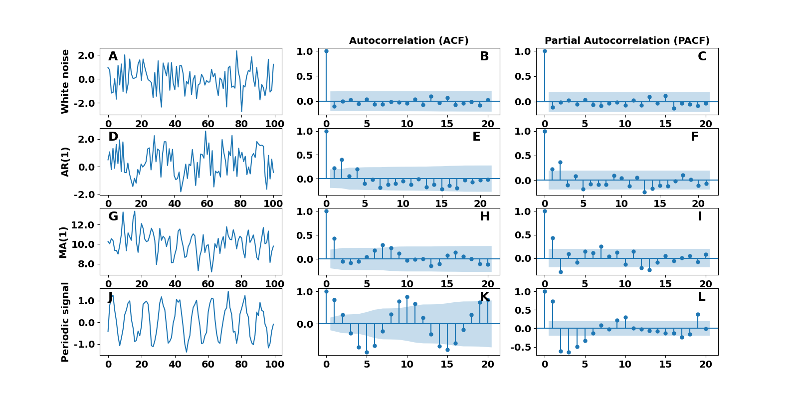
Figure 3. Estimation of ACF and PACF for three models. Each row shows a white noise, an AR(1), and a MA(1) raw data, the ACF, and the PACF. The blue-shaded area indicates the confidence interval cone ($ 95 $% confidence).
Let’s look now into a moving average model of order $ p = 1 $. In this case, the data shown in Figure 3G are described by the equation $ x[t] = 10 + 0.7 \epsilon[t-1] + \epsilon[t] $, which is MA(1) model. By examining the ACF plot in Figure 3H, we see strong correlations besides lag $ k = 0 $, which means that the data come from a process that is not completely random. In the PACF plot in Figure 3I, several lag components have strong correlations, and the PACF decays geometrically.
The final example regards a periodic time series with period $ T $. Figure 3J shows a sinusoidal signal $ g(t) = \sin(2 \pi t \frac{1}{T}) + \epsilon $ with additive white noise, $ \epsilon $, and $ T = \frac{1}{10} $. Because there are several components with strong correlations in the ACF and PACF plots, we know there is some structure in the data. The ACF plot in Figure 3K reflects the periodicity of the time series. We can infer that the signal’s frequency is $ f = 10 $ (where an entire cycle has been completed). Moreover, the lag component on the frequency ($ k = 10 $) is the strongest in the graph. Therefore, if we needed to know the frequency of the raw data without knowing the model, we could infer the period by looking into the ACF plot.
A few remarks on ACF and PACF plots
Let’s now draw some conclusions and remarks regarding the ACF and PACF and how to use them to identify an underlying model in raw data.
- When a time series (or a signal) contains a moving average term (MA), we can determine the exact order of the MA by counting the components with strong correlations in an ACF plot. That’s true even when the underlying model is a high-order MA.
- When the PACF plot has strong correlations up to some lag $ k > 0 $, there is an autoregressive term (AR) in the raw data. The number of those elements determines the order $ p $ of the AR($ p $) model.
- When a strong positive correlation exists and the PACF oscillates around zero, then there is a moving average, MA, term. The same holds when the zero lag is negative, and the PACF decays geometrically to zero.
- If the PACF shows strong correlations up to a lag $ k $ and then decays geometrically to zero, it suggests that the data can be effectively modeled by an ARMA(p, q) model.
Why do we need models like AR(p), MA(q), and others ?
So far, we have seen the ACF and PACF and how to estimate them, given a time series. Moreover, we have seen how to use the ACF and PACF plots to determine the parameters of models such as AR(p) or MA(q). However, there is one question we still need to answer. Why do we need models like AR(p) in the first place? The answer is to describe raw data with a mathematical model that will allow us to make predictions (forecasting) of future values of our system.
Let’s be more specific. Assume that we obtain some raw data (observations) like the ones in Figure 1 showing the number of airport passengers per month for the years $ 1949 - 1960 $. Suppose we would like to know the number of passengers in the next month or two months. In other words, we would like to predict the number of passengers in the future using known historical (past) observations.
One way to predict future values would be to assume that the number of passengers will keep growing following the current trend. However, that must be more accurate since we need a model for the underlying processes that describe our observations. A solution to that problem would be to apply the analysis we have already used. First, we would estimate the ACF and PACF and visualize the results. From ACF and PACF plots, we would find out the type of model (AR(p), MA(q), or other) that best fits our observations. Once we know that our observations follow a, let’s assume, AR(p) model with order $ p $, we can use that model to make predictions. More precisely, we could use equation (2) to fit the data and then the fitted equation to predict future values. Below, we provide Python code demonstrating how to make predictions using the statsmodels module.
First, let’s create the data set following an AR(1) model. For that reason, we will use the model in Figure 2D. The equation that describes the dynamics is $ x[t] = 0.6 * x[t-1] + \epsilon[t] $ (see the section about the AR(p) model). In a real-life situation, we won’t create the data set; instead, we will have to obtain it somehow.
In the first code snippet, we show how to build the data set from scratch.
 1import numpy as np
 2import matplotlib.pylab as plt
 3
 4from statsmodels.tsa.ar_model import AutoReg
 5
 6np.random.seed(3)	# fix the RNG seed for reproducibility
 7
 8# Create raw data using an AR(1) model
 9N = 1000 	# total number of observations
10x = [0.5]	# initial value
11for i in range(N):
12    x.append(0.6 * x[i-1] + np.random.normal(0, 1))
The next step is to split the raw data into two separate sets. One for training (fitting) the parameters of our AR model and one for testing the fitted model. The training data set is usually larger than the testing one. Therefore, we use $ 70 $% of the data for training and $ 30 $% for testing. Remember that we have already performed our analysis in Figures 2E and 2F, where we estimated the ACF and PACF. Thus, we know that the underlying process for those observations is an AR(1), and we need three lags to predict the future.
 1# Split the original data set into train/test data sets
 2K = int(N * 0.7)   # size of training data set
 3train_data = x[:K]
 4test_data = x[K:]
 5
 6# Fit the AR model using 3 lags (see Figures 2D, E, F)
 7# We use the same AR(1) model.
 8ARmodel = AutoReg(train_data, lags=3).fit()
 9
10# Print a summary of the fitting process
11print(ARmodel.summary())
Finally, we use the method predict of the class AutoReg to predict
five steps into the future (the horizon is five). As we see in Figure 4,
although the prediction is not perfect, it captures the main pattern.
1horizon = 5	# How many values into the future we want to predict
2prediction = ARmodel.predict(start=K, end=(K + horizon), dynamic=False)
3
4fig = plt.figure()
5ax = fig.add_subplot(111)
6ax.plot(prediction, 'b', label="prediction")
7ax.plot(test_data[:horizon], 'k', label="target")
8plt.plot()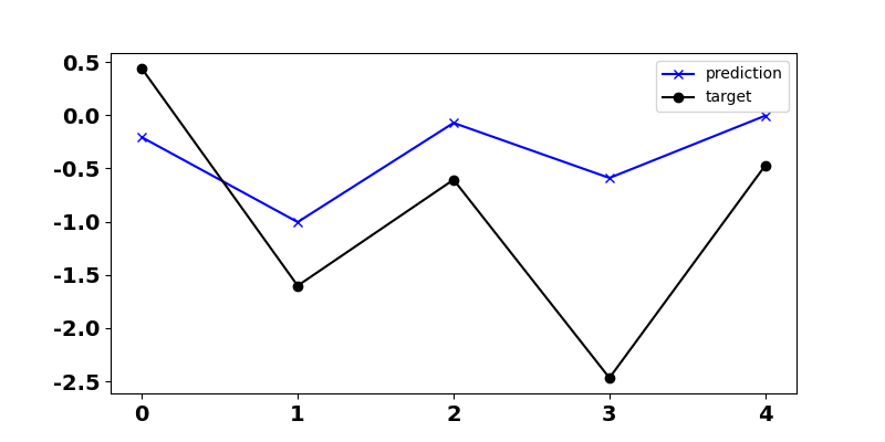
Figure 4. Prediction of an AR(1) process using statsmodels AutoReg. The black curve indicates actual observations and the red one is the predictions.
Summary
In this post, we defined the autocorrelation and the partial autocorrelation
functions, ACF and PACF. We introduced the AR(p), MA(q), ARMA(p, q), and ARIMA(p, d, q)
models, and we showed how one could use the ACF and PACF to determine the
parameters p, q, and d. Moreover, we provided a few examples and Python code
snippets on using the statsmodels acf and pacf functions. Finally,
we give a simple example of using AR(p) models to predict future values.
Cited as
@article{detorakis2022acfpacf,
  title   = "Autocorrelation functions for time series",
  author  = "Georgios Is. Detorakis",
  journal = "gdetor.github.io",
  year    = "2022",
  url     = "https://gdetor.github.io/posts/acf_pacf"
}
References
- J. Beran, Mathematical Foundations of Time Series Analysis A Concise Introduction, Springer, 2017.
- “Time series”, Wikipedia, Wikimedia Foundation, May 2 2022.
- “Autocorrelation”, Wikipedia, Wikimedia Foundation, May 2 2022.
- “Partial autocorrelation function”, Wikipedia, Wikimedia Foundation, May 2 2022.
- S. Wang, C. Li, and A. Lim, Why Are the ARIMA and SARIMA not Sufficient, arXiv:1904.07632, 2019.