Genetic Algorithms & Island Models
In this post, we explore genetic algorithms (GAs) and the so-called island model (IM). GAs and the IM are optimization methods used to maximize or minimize a cost function.
What is Optimization?
Let’s see an example of an optimization problem we all face every day. Let’s assume you’d like to go and grab a couple of coffee from your favorite coffee shop. Typically, you ask Google to find the fastest way to the store from your current location. But let’s forget about technology for now.
You only have a map. Yes, a paper map! They are still around! You first try to find the shortest paths from your current location to the coffee shop. If you’re a scrooge, you will define the “optimal path” as “the path I consume the least fuel.”
An optimization problem is a search for the “best” set of parameters, where “best” is defined as the minimum or maximum of some cost function of interest. Here, that function is our fuel consumption. However, we could have also designated it to be the distance from start to finish.
Mathematically speaking the problem of a minimization can be formulated as follows [1]: Given a function $f:A\subseteq \mathbb{R} \rightarrow \mathbb{R}$ we are searching for an element $ {\bf x}^* $ such that $$ f({\bf x}^*) \leq f({\bf x}) $$
for all $ {\bf x} \in A $. Similarly, a maximization would be the search for a ${\bf x}^* $ such that $$ f({\bf x}^*) \geq f({\bf x}) $$ for all $ {\bf x} \in A $.
In both cases, we are searching for a global optimum (either a global minimum or a global maximum). However, it is not always possible to find a global optimum point in real-life cases. Instead, we can settle for a local minimum or maximum. For example, that’s the compromise we often make when training neural networks with backpropagation [2].
Figure 1A shows the global minimum of the cost function, $f(x)=x^2$, with a magenta color. Figure 1B displays what is known as the Rastrigin function in one dimension. It is evident that this function has multiple local minima (e.g.,, magenta disc) and maxima (green disc) as well as one global minimum at $(0, 0)$ (black disc).
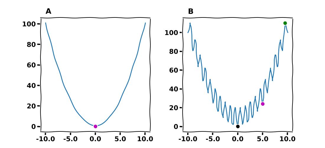
Figure 1. Global and local extremes for (A) $f(x)=x^2$, where the magenta disc indicates the global minimum at $(0, 0)$. (B) For Rastrigin $f(x) = 10 + x^2-10\cos(2\pi x)$, there is a global mimimum at $(0, 0)$ and many local mimima and maxima (for instance see the magenta and green discs, respectively).
Sometimes, it’s easier to solve a minimization problem from a computational standpoint. In that case, we would minimize the function $ -f $.
What is a Genetic Algorithm?
A genetic algorithm is an optimization method that mimics evolution to optimize a cost function. The entire set of the cost function parameters is called the genome. Each parameter consists of a gene. Because GA mimics how evolution works, they require a population of individuals. Each individual is nothing more than a randomly initialized genome. Any GA starts optimizing a cost function after initializing a population of genomes (individuals).
In most GA implementations, an individual is a a data structure that holds a genome (vector of bits, integers, floats, etc.), the corresponding cost to its genome, a unique ID, a flag indicating whether the current individual is about to mate (after a selection process), and other relevant information that the developer deems necessary.
When the GA optimizes a cost function, it usually applies three basic operators:
-
Selection This operator selects two individuals from a population (i.e., a set of many individuals) to mate and eventually procreate. The selected individuals are called parents. Some selection operators are k-tournament, roulette-wheel, random, etc.
-
Crossover This operator mises the genomes of the selected parents. A crossover operator will combine a part of the first parent’s genome with a part of the second parent’s genome. Some crossover operators are one-point crossover, two-points crossover, random, etc.
-
Mutation Finally, the potential offspring’s (or child’s) genome is subject to a mutation, which will further change the offspring’s genome. Some of the most used mutation operators are delta, random, etc.
Typically, a GA will repeat every generation’s operations mentioned above (another fancy term for iteration). At every iteration, potential offspring will replace their parents. Usually, the best-performing offspring will replace the most poor-performing parents in terms of fitness. We call that kind of replacement “elite” replacement. Another idea of replacing the parents is randomly choosing some of the parents and replacing them.
When the GA exhausts the predefined number of generations, the algorithm terminates. We can evaluate its performance by inspecting the average fitness (the average cost function value over all the individuals) or the best-so-far fitness (BSF). Figure 2A shows a typical example of average fitness and 2B a BSF. Upon the algorithm’s termination, the individual with the best fitness function provides the genome (set of parameters) optimizes the cost function [3].
How a Genetic Algorithm works?
Let’s use an example to try to understand how GAs work.
Example
Let’s try to solve the XOR problem using a feed-forward neural network. The XOR (exclusive OR) is a binary operator that returns true if and only if the operands are different. This means that if $ X = 1 $ (or $ X = 0 $) and $ Y = 0 $ (or $ Y = 1 $) then $ X \oplus Y = 1 $ (same when ). If both $ X $ and $ Y $ are zeros or ones, then $ X \oplus Y = 0 $.
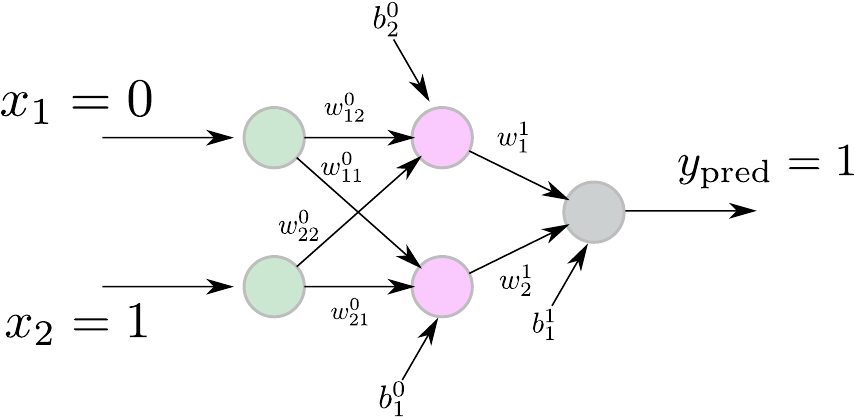
Figure 2. XOR neural networ.
Our neural network will consist of two input units (since the XOR operator is a binary one), two hidden units, and one output unit. Please see here for more details on why we choose such an architecture. Figure 2 shows the neural network we are about to use. Let’s optimize this neural network that will serve as an XOR operator. To facilitate the demonstration, let’s split the process into four steps:
-
Define the cost function and the size of our genome. Since the input to the XOR function is two-dimensional, we have a genome of size two. Regarding the cost function, we first define an error term as $$ \epsilon = | y_{\text{target} - y_{\text{pred}}} | $$ where $ y_{\text{target}} $ is the true value that the XOR function returns and $x_{\text{pred}}$ is the value of our network’s output. Since we have four pairs of inputs $ (0, 1), (1, 0), (1, 1), (0, 0) $, and four real outputs $1, 1, 0, 0$, respectively, we define the cost function as: $$ f({\bf x}) = \sum_{i=1}^{4} \epsilon_i $$ Ideally, we expect the cost function to be zero to get our optimal solution. That’s the case in Figure 2, where we see the best-so-far fitness and the average fitness.
-
Once we have defined the cost function (that’s always the most challenging part), we determine the number of genes per individual, which is $9$ in this case. The neural network has the two input units connected via a $ 2 \times 2 $ matrix with the two hidden units. Next, the hidden units connect via a $ 2\times 1 $ matrix to the output unit. Moreover, the hidden and output units have a bias term (3 bias terms in total). Therefore, the entire network has nine parameters (six weights and three bias terms) we have to optimize. So, we initialize the neural network with small random weights, define the number of individuals (population size) to be $ 20 $, and define the size of the genome to be $ 9 $. Remember, this is the number of cost function parameters to optimize. We set the number of generations to $ 5000 $, the number of offspring to $ 10 $, and the replacement size to $ 5 $, which means $ 5 $ parents will be replaced by $ 5 $ offsprings.
-
We need to decide what operators we will use for our GA. In this particular example, we use a k-tournament selection, a one-point crossover, and a delta mutation operator.
- k-tournament selection This operator will randomly choose $ k $ individuals from the population. It will, then, choose the best individual, based on the fitness from the tournament with probability $ p $, choose the second-best individual with probability $ p(1-p) $, the third-best with probability $ p(1-p)^2 $, etc.
- One-point crossover will take the genes of two parents as input, it will randomly pick a number from zero to the size of genes, and it will cut the parents’ genes at that point. Then it will swap the sliced genes between the two parents, and thus the offspring will carry genetic information from both parents.
- Delta mutation operator will draw uniformly a number from the interval $ [0, 1] $ for each gene in an individual’s genome. If that number is greater than a probability $ p $ (usually $ p = \frac{1}{2} $). A predefined increment will increase the value of the gene.
-
Finally, we set our Optimization in motion. The GA will first evaluate the cost function of each individual. It will sort the individuals based on their fitness values. To this end, we feed the XOR input to the neural network, and we collect the output $ y_{\text{pred}} $. Then we use the output to compute the cost function value for that individual. The next step for our GA is to choose two parents based on the k-tournament selection. The genome of the two selected parents will be crossed over using the one-point operator. That will give rise to a new genome, a child or offspring. The offspring’s genome will undergo a mutation based on the delta operator. Finally, the GA will add the offspring to a list. The selection, crossover, and mutation processes continue until the number of offspring have been exhausted. Then, the best performing offspring will replace the poorest-performing (maximum cost function value) parents (elite replacement). And the entire process repeats for $ 4999$ more generations.
After the convergence of the process described in step $ 4 $, the Optimization of the XOR fitness terminates, and we can inspect the results. Figure 3 shows the best-so-far fitness (BSF) and the average fitness, respectively. The first observation is that the cost function value indeed converges to zero. Thus, our GA’s best genome is optimal, and our neural network solves the XOR problem. The second observation is that we could have used only $500$ generations for this particular instance. The difficulty of the problem at hand usually determines the number of generations and the initial values of the genome.
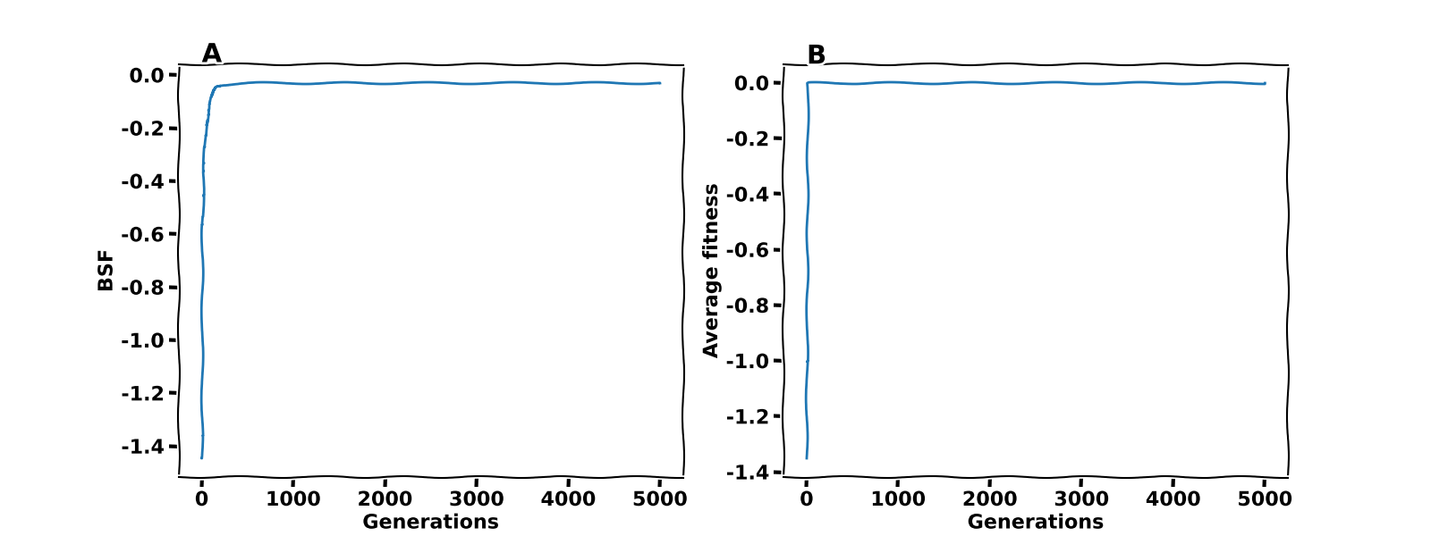
Figure 3. BSF and average fitness for the optimization of the XOR fitness function.
Bellow, you can find the source code of the Python script we used to optimize the XOR problem. As you can see, we combine Pytorch and PyGAIM to build a neural network and optimize the weights and the biases.
The first snippet shows what packages we need to import, the class of the neural network, and a function that we will use to measure the accuracy of our optimization process.
 1import sys
 2import numpy as np
 3import matplotlib.pylab as plt
 4from random import shuffle
 5
 6import torch
 7from torch import nn
 8
 9sys.path.append("/home/gdetorak/packages/gaim/pygaim")
10from pygaim import GAOptimize, c2numpy
11
12
13class XOR_NET(nn.Module):
14    def __init__(self):
15        super(XOR_NET, self).__init__()
16
17        self.fc1 = nn.Linear(2, 2)
18        self.fc2 = nn.Linear(2, 1)
19        self.sigmoid = nn.Sigmoid()
20
21    def forward(self, x):
22        out = self.sigmoid(self.fc1(x))
23        out = self.fc2(out)
24        return out
25
26# Instantiate the XOR_NET class
27net = XOR_NET()
28
29# src: Input XOR
30# tgt: Output XOR
31src = np.array([[0, 1], [1, 0], [1, 1], [0, 0]], 'f')
32dst = np.array([[1], [1], [0], [0]], 'f')
33index = [0, 1, 2, 3]
34
35
36def accuracy(genome):
37    """
38    Measures the accuracy of the XOR_NET. Runs over 100 times
39    and compares the network output against the target pattern
40    each time.
41    """
42    # Assign genomes to network weights
43    w1 = genome[:4]
44    b1 = genome[4:6]
45    w2 = genome[6:8]
46    b2 = genome[8:]
47
48    net.fc1.weight.data = torch.FloatTensor(w1).reshape(2, 2)
49    net.fc1.bias.data = torch.FloatTensor(b1)
50    net.fc2.weight.data = torch.FloatTensor(w2).reshape(1, 2)
51    net.fc1.bias.data = torch.FloatTensor(b2)
52
53    count = 0
54    for i in range(100):
55        idx = np.random.randint(0, 4)
56        inp = torch.FloatTensor(src[idx])
57        tgt = torch.FloatTensor(dst[idx])
58        y = net(inp)
59        if np.round(y.item()) == np.round(tgt.item()):
60            count += 1
61            # print(y.item(), tgt.item())
62    print("Accuracy: %d / 100" % count)
The fitness function takes the genome (C array) as input and returns the negative of fitness value (or loss) since we perform a minimization. It presents each time all four XOR patterns to the neural network and computes the loss for each pattern. Finally, it sums up all four individual losses and returns the total loss.
 1def fitness(x, length):
 2    """
 3    Fitness function. Receives the genome (x) from GAIM, passes it through
 4    net.forward (Pytorch) and computes the absolute loss.
 5    """
 6    x = c2numpy(x, length)				# Convert C array to Numpy
 7    w1 = x[:4]						# First layer weights (2x2)
 8    b1 = x[4:6]					# First layer bias (2X1)
 9    w2 = x[6:8]					# Second layer weights (2x1)
10    b2 = x[8:]						# Second layer bias (1x1)
11
12    # Assign the new values to network weights
13    net.fc1.weight.data = torch.FloatTensor(w1).reshape(2, 2)
14    net.fc1.bias.data = torch.FloatTensor(b1)
15    net.fc2.weight.data = torch.FloatTensor(w2).reshape(1, 2)
16    net.fc1.bias.data = torch.FloatTensor(b2)
17
18    loss = 0.0
19    shuffle(index)					# shuffle the index
20    # loop over all four patterns in a random order
21    for idx in index:
22        inp = torch.from_numpy(src[idx])
23        tgt = torch.from_numpy(dst[idx])
24        y = net(inp)
25        loss += torch.abs(y[0] - tgt[0])
26 return float(-loss.item()) # return -loss (minimize) 1 genome_size = 9
2 ga = GAOptimize(fitness,
3 n_generations=1000,
4 population_size=10,
5 genome_size=genome_size,
6 n_offsprings=5,
7 n_replacements=2,
8 a=[float(-10.0) for _ in range(genome_size)],
9 b=[float(10.0) for _ in range(genome_size)],
10 mutation_rate=0.5,
11 mutation_var=.1)
12 genome, _, _ = ga.fit()
13 ga.plot_()
14 test_weights(genome)
15 plt.show()For more information about GAIM, its source code, and examples, you can visit its Github repository.
What is an Island Model?
An island model is a computational method that runs multiple instances of GAs on the same optimization problem in a distributed and parallel fashion. In some cases, each island (another fancy word for process, thread, or computational node in a cluster) can run a part of the optimization problem [5].
What is essential in an island model is the periodic exchange of individuals between islands. According to a predetermined time interval, a migration of a subpopulation takes place. This circulation of individuals between islands relies on specific communication protocols and predetermined topologies (e.g., ring topology). In this case, the islands are connected, forming a ring, meaning the current island (node) connects to the one on its right (or left).
Figure 4 shows three basic topologies, (A) all-to-all, where every island connects to all other ones, (B) ring, and (C) star topology, where one island serves as a communication hub [5, 6, 7].
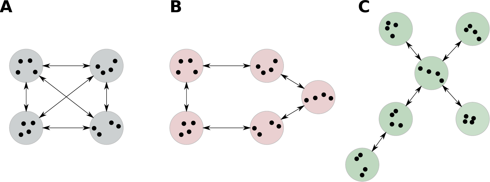
Figure 4. Island model topologies. (A) all-to-all, (B) ring, (C) star.
Each island begins with a population of $N$ individuals where $$ N = \frac{K}{M} $$ where $ K $ is the number of all individuals, and $M$ is the number of islands. Every island will initialize a GA based on all the parameters and procedures described earlier. When a time counter exhausts, migration takes place. The IM algorithm selects a subpopulation on each island via some selection method (random, elite - the best performing individuals, etc.). The selected genomes move to the neighboring, connected island or islands. The newly arrived ones replace local individuals via a replacement method (random, poor - the worst-performing individuals, etc.). IM fills the vacant spots on the source island with new offspring or randomly generated individuals [6]. The number of individuals moved at every migration interval is called the “migration size.” The reader can refer to [8, 9] for more information on how the migration interval and the migration size affect the performance of an island model.
The island model offers a means of faster convergence since each island can potentially follow a different evolutionary trajectory covering different parts of the search space. Furthermore, exchanging individuals between islands can help the overall optimization process avoid being stuck in some local minimum/maximum. That doesn’t mean that the island model is impervious to local extrema.
When should we use GAs?
As we have seen, GAs can optimize virtually any function given a well-defined cost function (and that’s the most challenging part of using GAs). However, there are some cases where we should try to use a GA instead of any other conventional optimization method. These instances are:
- If the search space is massive, then GAs are suitable for optimizing a function in that space (for instance, non-linear functions).
- Another issue with Optimization is the cost function. The cost function may be discontinuous (having gaps), or it may be non-differentiable. GAs do not use derivatives and are therefore immune to such issues.
- When a cost function is too complex, GAs have more chances than the vanilla optimization methods to avoid local minima and correctly find the global optimum. A genetic algorithm can simultaneously explore the search space in multiple directions, even if some offspring will never discover an optimal solution to the problem.
- Finally, GAs are agnostic to the problem at hand. They do not require any information about the system or the function they optimize to solve the optimization problem.
What are some of the GAs applications?
Here, you can find some of the GA’s applications in real life. Although the the following list is not complete; you will glimpse where and how GAs are used.
- Optimization As discussed in this post, GAs can optimize almost any function.
- Machine learning GAs can tune ML/DL models to discover optimal neural network parameters. Moreover, they can design neural networks (searching for the optimal neural network topology [10]).
- Path and trajectory planning GAs can aid in the designing and planning of paths and trajectories for autonomous robotic platforms, vehicles, or manipulators, such as robotic arms.
- DNA Analysis GAs can analyze the structure of DNA samples.
- Finance GAs are an excellent tool for analyzing and forecasting stock prices.
- Aerospace engineering GAs can aid in the process of designing aircraft.
- Traveling salesman problem (TSP) The TSP is well-defined in combinatorial Optimization and has many applications in real-life issues.
Cited as:
@article{detorakis2022geneticalg,
  title   = "Genetic algorithms and island models",
  author  = "Georgios Is. Detorakis",
  journal = "gdetor.github.io",
  year    = "2022",
  url     = "https://gdetor.github.io/posts/genetics_algorithms"
}
References
- D. A. Pierre, Optimization theory with applications, Courier Corporation, 1986.
- I. Goodfellow, B. Yoshua, and A. Courville, Deep learning, MIT press, 2016.
- K. De Jong, Evolutionary computation, Wiley Interdisciplinary Reviews: Computational Statistics, 2009, 1.1: 52-56.
- G. Is. Detorakis and A. Burton, GAIM: A C++ library for Genetic Algorithms and Island Models, Journal of Open Source Software, 2019, 4.44: 1839.
- D. Whitley, S. Rana, and R.B. Heckendorn, The island model genetic algorithm: On separability, population size and convergence, Journal of computing and information technology, 7:1, 33–47, 1999.
- D. Sudholt, Parallel evolutionary algorithms, Springer Handbook of Computational Intelligence, 929–959, 2015.
- W. N. Martin, J. Lienig, and J. P. Cohoon, Parallel Genetic Algorithms Based on Punctuated Equilibria, Handbook of Evolutionary Computation, IOP Publishing group, 1997.
- Z. Skolicki, An analysis of island models in evolutionary computation, Proceedings of the 7th annual workshop on Genetic and evolutionary computation, 386–389, 2005.
- Z. Skolicki, and K. De Jong, The influence of migration sizes and intervals on island models, Proceedings of the 7th annual conference on genetic and evolutionary computation, 1295–1302, 2005.
- K. O. Stanley, and R. Miikkulainen, Efficient evolution of neural network topologies, Proceedings of the 2002 Congress on Evolutionary Computation. 2, 1757–1762, 2002.