Time series forecasting error metrics
In this post, we will explore the basic error measures used in time-series forecasting. Error measures provide a way to quantify the quality of a forecasting algorithm (e.g., the performance). First, we briefly introduce time series and the fundamental terms of forecasting. Second, we will introduce the most commonly used error measures and give examples. Finally, we provide a complete example of using errors in a real-life forecasting scenario.
What is a time series
A time series is a series of data points indexed in time order in layman’s terms [1, 2]. A few examples of time series are
- The daily closing price of a stock in the stock market
- The number of air passengers per month
- The biosignals recorded from electroencephalogram or electrocardiogram
Figure 1 shows the number of air passengers per month from January 1949 to September 1960. You can download the data from Kaggle here.
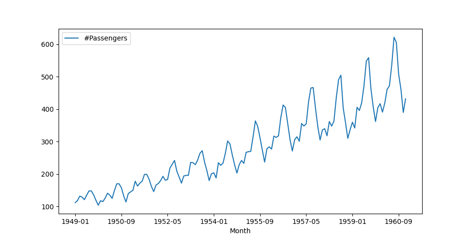
Figure 1. An example of a time series showing the number of air passengers per month.
A more rigorous definition of a time series found in [1] (Chapter 1, pg 1) is given below:
Let $ k \in \mathbf{N}, T \subseteq \mathbf{R} $. A function $$ x: T \rightarrow \mathbf{R}^k, \hspace{2mm} t \rightarrow x_t $$ or equivalently, a set of indexed elements of $ \mathbf{R}^k $, $$ { x_t | x_t \in \mathbf{R}^k, \hspace{2mm} t \in T } $$ is called an observed time series (or time series). Sometimes, we write $ x_t(t \in T) $ or $ (x_t)_{t\in T} $.
When $ k = 1 $ the time series is called univariate, otherwise is called multivariate. $ T $ determines if the time series is [1]:
- discrete $ T $ is countable, and $ \forall a < b \in \mathbb{R}: T \cap[a, b] $ is finite,
- continuous $ T = [a, b], a < b \in \mathbb{R}, T = \mathbb{R}_{+} \hspace{2mm} \text{or} \hspace{2mm} T = \mathbb{R} $,
- equidistant $ T $ is discrete, and $ \exists u \hspace{2mm} s.t. \hspace{2mm} t_{j+1} - t_j = u $.
From now on and for simplicity’s sake we will use the following notation for a time series: $ y[1], y[2], \ldots , y[N] $, where $ N \in \mathbb{N} $ or $ y[t] $, where $t=1, \ldots , N $.
More terminology
Before we dive into the post, let’s give some valuable terminology for the unfamiliar reader.
- Observed data ($ (y_t)_{t\in T} $ or $ y[t] $) This is the data we obtain by observing a system or a process.
- Predictive model Is a mathematical representation of observed data.
- Target ($ y[t] $) This is the ground truth signal we use to train a predictor.
- Horizon ($ h $) Is the number of points or steps we predict in the future.
- Prediction ($ \hat{y}[t] = y[t+h] $) This is a value that predictor returns.
- Forecasting Is the process of predicting future values from historical and present data.
- Outlier This value significantly differs from other time series values.
- Error ($ \epsilon[t] $) is the difference between the target signal and the prediction of our model. The error is given by $ \epsilon[t] = y[t] - \hat{y}[t] $.
- Seasonality ($ S $) Seasonality is the periodic appearance of specific patterns over the same period—for instance, increasing prices before and over the Christmas holidays.
Four basic predictors
So far, we have seen what a time series is and the basic terminology. Now, we will explore some essential predictors or models and see how to use them to forecast.
As we’ve already seen, a predictor is a statistical (or mathematical) model that receives as input historical and present data and returns one (one-step ahead forecasting, $ h = 1$) or multiple future values (multi-step ahead prediction, $ h > 1 $). The development of predictors is out of the scope of this post, so we will not see how to build, train, test/validate, and use a predictor (here are a few references where the reader can find more details on that matter [3, 4, 5, 6]). However, we will introduce the four elementary predictors since some error measures use some of them to estimate the prediction errors.
Naive predictor
The most straightforward predictor we can imagine is the naive one. It takes the last observed value and returns it as the predicted value:
$$ \hat{y}[t + h | t] = y[t]. $$
Seasonal predictor
We can use the seasonal predictor when we know that our time series has a seasonal component (seasonality). It is a natural extension of the naive one, and we can describe it as:
$$ \hat{y}[t+h|t] = y[t+h-S(P+1)]. $$
$ P $ is $ \Big[\frac{h-1}{S}\Big] $, where $ \Big[ x \Big] $ is the integer part of $ x $. $ P $ reflects the number of years–365 days– have passed prior to time $ t + h $.
Average predictor
This predictor receives historical and present values as input, computes their average (or mean), and returns it as a prediction:
$$ \hat{y}[t+h|t] = \bar{y} = \frac{1}{N} \sum_{t=1}^{N} y[t] .$$
Drift predictor
Another variation of the naive predictor, only this time we allow to the predicted value to drift (fluctuate) over time,
$$ \hat{y}[t+h|t] = y[t] + \frac{h}{t-1} \sum_{j=2}^{t} (y[j]-y[j-1]) = y[t] + h\Big( \frac{y[t] - y[1]}{t - 1} \Big). $$
You can picture this predictor as a line drawn from the first observation to the last one and beyond, where beyond is the prediction.
Figure 2 shows the predictions in each of the cases mentioned above for the air passenger data (brown line). The blue line represents the naive predictor, the green line represents the seasonal predictor, the orange line represents the average predictor, and the pink line indicates the drift predictor.
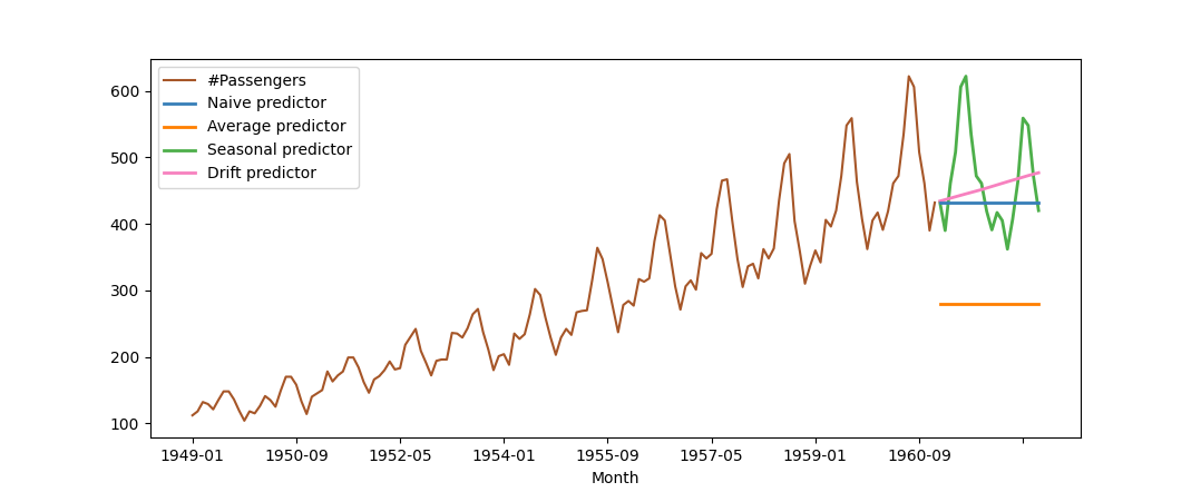
Figure 2. Forecasts of montly air passengers. Naive predictor (blue line), naive seasonal (green), average (orange), drift (pink).
Forecasting error measures
So why do we need error measures? The general idea is to quantify the distance between an actual observation (target) and a predicted one. Particularly when we train a model to learn how to predict future values, we have to measure the error between the actual and predicted observations. Hence, minimizing the error leads to a better model.
When we teach a model, we need to use penalties to help it improve its predictions. The error measures listed below do precisely that. They measure how far the model’s predictions are from the ground truth and penalize the model accordingly. Usually, the smaller the error, the better the predictor.
Another reason we need error measures is to evaluate the performance of our model in real-life scenarios. We might have a trained model that performs some forecasting, and we would like to investigate the quality of its predictions. In this case, we can measure the error between the historical data we will collect in the future and the model’s predictions.
We already said that developing and training a predictor is out of the scope of the present post. Therefore, we will use historical data and add Gaussian noise to fake the predictions. Furthermore, we adopt the discrete-time signals time indexing, meaning that $ y[t] $ is the time series value at time index $ t $. A similar way would be $ y_t $, where $ t $ is the time index.
Reminder $ y[t] $ is the target signal, $ \hat{y}[t] $ the prediction signal and $ \epsilon[t] $ the error signal.
And now, we are ready to introduce the error measures and some examples demonstrating their behavior.
Example
In the following sections, we use some basic examples to demonstrate how the reader can implement the error measures in Python. In every case, we provide a custom implementation of the error measure and a Sklearn one. The reader should rely more on the Sklearn [7] implementation since it’s generic and optimized. We provide a custom implementation so the reader can better understand the mathematical formulas.
1import numpy as np
2np.random.seed(13)
3
4y_true = np.array([1.5, -0.5, 2.5, 3, 2, 1])        # This is y (target)
5
6y_pred = np.array([1, -0.3, 2.6, 3, 2.4, 1.2])      # This is y_hat (prediction)
Mean Absolute Error (MAE)
The MAE is the most straightforward error measure, and as its name signifies, it is just the difference between a target (or desired) value and model’s prediction. MAE is defined as:
$$ \frac{1}{N} \sum_{t=1}^{N} |y[t] - \hat{y}[t]| = \frac{1}{N} \sum_{t=1}^{N} | \epsilon[t] |. $$
By observing the definition of MAE, we can see that MAE is scale-dependent, meaning that both signals, target and prediction, must be of the same scale. However, MAE is robust to outliers. (see [8, 9] for ways to handle outliers and fix related issues).
Example
 1from sklearn.metrics import mean_absolute_error
 2
 3def MAE(y_true, y_pred):
 4    N = len(y_true)
 5    error = np.abs(y_true - y_pred).sum()
 6    return error / N
 7
 8print(MAE(y, y_hat))
 90.2333333333333333
10
11print(mean_absolute_error(y, y_hat))
120.2333333333333333
Mean Absolute Percentage Error (MAPE)
MAPE computes the error between a target and a prediction signal as a ratio of the error $ \epsilon[t] $ and the target signal. More precisely,
$$ MAPE = \frac{100\%}{N} \sum_{t=1}^{N} \frac{|y[t] - \hat{y}[t]|}{|y[t]|} = \frac{100}{N} \sum_{t=1}^{N} \frac{| \epsilon[t] |}{| y[t] |}. $$
MAPE is a helpful error measure when it serves as a loss function in training and validating a regression model [10]. This error measure is not susceptible to global scaling of the target signal.
Again, we can draw some conclusions about this measure by observing the definition of MAPE above. MAPE can be problematic when the actual values are zero or near zero. We can see from the definition above that when the denominator is close to zero or zero, the MAPE is too large or cannot be defined. Moreover, MAPE is susceptible to skewness since the term $ \frac{1}{y[t]} $ depends only on the observed data (not on the model’s predictions).
Example
 1from sklearn.metrics import mean_absolute_percentage_error
 2
 3def MAPE(y_true, y_pred):
 4    N = len(y_true)
 5    error = (np.abs(y_true - y_pred) / np.abs(y_true)).sum()
 6    return (100.0 / N) * error
 7
 8print(MAPE(y, y_hat))
 919.5555555555555557                 # this is because we multiply by 100
10
11print(mean_absolute_percentage_error(y, y_hat))
120.19555555555555554
13
Mean Squared Error (MSE)
The MSE is one of the most used error measures in Machine and Deep learning. It computes the average of the square of the errors between target and prediction signals. We define the MSE as:
$$ MSE = \frac{1}{N} \sum_{t=1}^{N} (y[t] - \hat{y}[t])^2 = \frac{1}{N} \sum_{t=1}^{N} \epsilon[t]^2 . $$
If we take the square root of $ MSE $, we get the Root MSE or RMSE. When the MSE is zero, we call the predictor (model) a perfect predictor. MSE falls into the category of quadratic errors. Quadratic errors tend to exaggerate the difference between the target and the model’s prediction, rendering them suitable for training models since the penalty applied to the model will be more prominent when the error signal is significant [11].
MSE combines the bias and the variance of a prediction. More precisely, $ MSE = b^2 + Var $, where $b$ is the bias term and $ Var $ is the variance. The bias reflects the assumptions the model makes to simplify finding answers. The more assumptions a model makes, the larger the bias. On the other hand, variance refers to how the answers given by the model are subject to change when we present different training/testing data to the model. Usually, linear models such as Linear Regression and Logistic Regression has high bias and low variance. Nonlinear models such as Decision Trees, SVM, and kNN have low bias and high variance [12]. Ideally, we would like to find a balance between bias and variance. That’s why sometimes we have to penalize our model during training using regularization techniques (this is out of the scope of the present post).
Example
 1from sklearn.metrics import mean_squared_error
 2
 3def MSE(y_true, y_pred):
 4    N = len(y_true)
 5    error = ((y_true - y_pred)**2).sum()
 6    return error / N
 7
 8print(MSE(y_true, y_pred))
 90.08333333333333333
10
11print(mean_squared_error(y_true, y_pred))
120.08333333333333333
Symmetric Mean Absolute Percentage Error (SMAPE)
SMAPE computes the error between the target and the prediction signals as a ratio of the error with the sum of the absolute values of actual and prediction values. The mathematical definition for SMAPE is:
$$ SMAPE = \frac{100\%}{N} \sum_{t=1}^{N} \frac{| \epsilon [t] |}{(| y[t]| + | \hat{y}[t] |)} $$
And as we can see from that definition, SMAPE is bounded from above and below, $ 0 \leq SMAPE \leq 100 $. Another remark we can make based on SMAPE’s definition is that when both a target and a prediction value are zero, the SMAPE is not defined. If only the actual or target value is zero, $ SMAPE = 100 $. Finally, SMAPE can cause troubles when, let’s say, a prediction is $ \hat{y}[t] = 10 $ the first time and $ \hat{y}[t] = 12 $ the second time, while in both cases, the target (actual) value is $ y[t] = 11 $. In the former case, $ SMAPE = 4.7 % $ and in the latter case $ SMAPE = 4.3 % $. We see that we get two different error values for the same target when our predictor returns different predictions.
Mean Absolute Scaled Error (MASE)
MASE is a metric that computes the error ratio between the target and the model’s prediction to a naive predictor’s error (forecaster).
The following equation gives the MASE,
$$ MASE = \frac{\frac{1}{N} \sum_{t=1}^{N} | \epsilon[t] | }{\frac{1}{N-1} \sum_{t=2}^{N} | y[t] - y[t-1] | } $$
When we are dealing with time series with seasonality with period $ S $ we can use the following MASE formula instead:
$$ MASE = \frac{\frac{1}{N} \sum_{t=1}^{N} | \epsilon[t] | }{\frac{1}{N-S} \sum_{t=S+1}^{N} | y[t] - y[t-S] | }. $$
MASE is scale-invariant, meaning that it’s immune to any scaling we perform on the observed data. MASE is symmetric, which implies that it penalizes both positive and negative (as well as big and small) forecast errors equally. When the MASE error exceeds one, the naive forecaster performs better than our model. MASE can only be problematic when the actual (target) signal has zero values. In that case, the naive predictor will be zero ad infinitum; thus, the MASE will be undefined.
Coefficient of Determination (CoD) or R²
The $ R^2 $ or Coefficient of Determination is an error measure frequently used in evaluating regression models (goodness of fit or best-fit line). $ R^2 $ counts how many of the target data points approach the line formed by the regression [11].
We define $ R^2 $ as
$$ R^2 = 1 - \frac{\sum_{t=1}^{N}(y[t] - \hat{y}[t])^2 }{\sum_{t=1}^{N}(y[t] - \bar{y})^2} = 1 - \frac{MSE}{Var[y[t]]}, $$
or alternatively
$$ R^2 = \frac{SSR}{SST} = \frac{\sum_{t=1}^{N}(y[t] - \hat{y}[t])^2 }{\sum_{t=1}^{N}(y[t] - \bar{y})^2}. $$
SSR is the sum of squares regression, and SST is the sum of squares total. SSR represents the total variation of all the predicted values found on the regression plane from the mean value of all the values of response variables. SST reflects the total variation of actual values (targets) from the mean value of all the values of response variables.
$R^2$ is bounded from above, $R^2 \leq 1$, since the fraction term lives always in the interval $ [0, 1] $. In the case of training, a regression model $ R^2 $ is bounded from bellow $ 0 \leq R^2 \leq 1 $. For the test/validation data, $ R^2 $ can be negative when MSE is large, or the total variance of the target (actual) signal is too small. A negative $ R^2 $ implies that the term $ \bar{y} $ is a better predictor than our model. Moreover, from the first definition of $ R^2 $, we see a direct relation between $ R^2 $ and MSE. While the $ R^2 $ increases, the MSE tends to approach zero. When we have an ideal predictor, $ MSE = 0 $ and $ r^2 = 1 $.
Example
 1from sklearn.metrics import r2_score
 2from numpy import var
 3
 4def R2(y_true, y_pred):
 5    mse = MSE(y_true, y_pred)
 6    variance = var(y_true)
 7    return 1.0 - (mse / var)
 8
 9print(R2(y_true, y_pred))
100.9351351351351351
11
12print(r2_score(y_true, y_pred))
130.9351351351351351
Summary
In this post, we briefly introduced the concept of time series and the most frequently used error measures in forecasting. We described the pros and cons of each measure so the reader can decide which one best suits their needs. If you find any typos or errors, or you have any other comments, please feel free to report them (you can find contact information here).
Cited as:
@article{detorakis2022errors-timeseries,
  title   = "Time series and forecasting error measures",
  author  = "Georgios Is. Detorakis",
  journal = "gdetor.github.io",
  year    = "2022",
  url     = "https://gdetor.github.io/posts/errors"
}
References
- J. Beran, Mathematical Foundations of Time Series Analysis A Concise Introduction, Springer, 2017.
- “Time series”, Wikipedia, Wikimedia Foundation, May 2 2022.
- A. Nielsen, Practical time series analysis: Prediction with statistics and machine learning, O’Reilly Media, 2019.
- R. J. Hyndman, and G. Athanasopoulos, Forecasting: principles and practice, OTexts, 2018.
- D. Oliveira, Deep learning for time series forecasting, https://www.kaggle.com/code/dimitreoliveira/deep-learning-for-time-series-forecasting, Kaggle, 2019.
- R. Mulla, [Tutorial] TIme series forecasting with XGBoost, https://www.kaggle.com/code/robikscube/tutorial-time-series-forecasting-with-xgboost, Kaggle, 2019.
- Pedregosa, F. et al., Scikit-learn: Machine Learning in Python, Journal of Machine Learning Research, 12, 2825–2830, 2011.
- F. Grubbs, Sample Criteria for Testing Outlying Observations, Annals of Mathematical Statistics 21(1):27–58, DOI:10.1214/aoms/1177729885, 1950.
- B. Rosner, Percentage Points for a Generalized ESD Many-Outlier Procedure, Technometrics 25(2):165–172, 1983.
- A. de Myttenaere, B. Golden, B. Le Grand, and F. Rossi, Mean absolute percentage error for regression models, Neurocomputing, 2016.
- A. Kumar, Mean squared error or R-squared - Which one to use? https://vitalflux.com/mean-square-error-r-squared-which-one-to-use/, 2022.
- C. M. Bishop, and N. M. Nasrabadi, Pattern recognition and machine learning, New York: Springer, 2006.